Neural Network with Numpy

Recommendations: This blog shows some mathematical expressions that looks bad in dark theme, It's recommended to read this blog in light theme.

Content

• introduction
• What is NumPy?
• Starting
  • tools
  • environment
• coding
  • Neural network and perceptron
  • Layer
  • Activation function
  • Neural Network Model
  • Testing our model
  • Training the model
  • Calculation of losses
  • Calculation of gradients
  • Training cycles
  • Testing our model with real data
• Source code

Introduction

Welcome, in this blog I will teach you to program a neural network in a few code lines using only the Numpy library.

It is recommended that you have previous basic knowledge of python, numpy and a bit of lineal algebra.

What is NumPy?

Numpy is a library for the Python programming language that supports creating large multidimensional arrays and vectors, along with a large collection of high-level mathematical functions to operate on them.
More info Here.

Starting.

Tools

• Python 3: First we need to install python, any version> 3.5 will do, in this case we will use Python 3.8
  On another occasion I will blog on how to install python correctly, for now you should find out how to do it.
• A code editor: You can use the one you like the most, here some examples: Visual code, Atom

Environment

We will use a virtual environment to facilitate things using virtualenv that is already included in the python installation.

For create a virtual environment run this in your terminal.

# We first create our project folder.
mkdir neural_network 

# We move to the folder.
cd neural_network

# This creates the virtual environment in my_env folder
python3 -m venv my_env 

For activate the virtual environment run.

source my_env/bin/activate

Now we are going to install the Numpy library in the virtual environment.

# upgrade the pip
pip install -u pip

#install numpy library
pip install numpy

Coding

Neural network and perceptron

A neural network is made up of functions like artificial neurons or perceptrons.

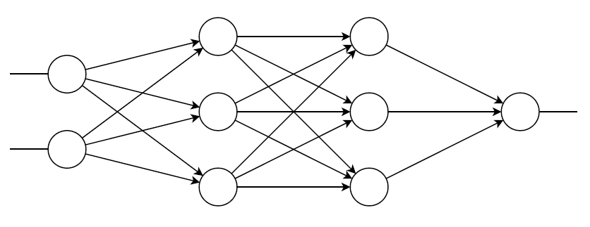
A perceptron is composed of a linear function, and an activation function.

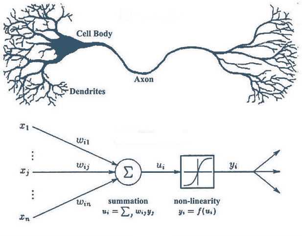
Mathematically the perceptron would look like this:

• y = f(wx + b)

• "x" is the data or signal it receives from another neuron
• "w" is the weight that the signal received will have.
• "b" is the bias of the neuron that corrects the prediction, in a linear equation "y" = "b" when all "x" is equal to 0.
  In our implementation we will calculate the predictions in this way.
• "f()", is the activation function, then we explain about this

The variables "w" and "b" control the result of the output "y". See this example

where:

• "X,W,B" are matrix
• "m" is the input examples number
• "i" is the inputs number
• "n" is the outputs number

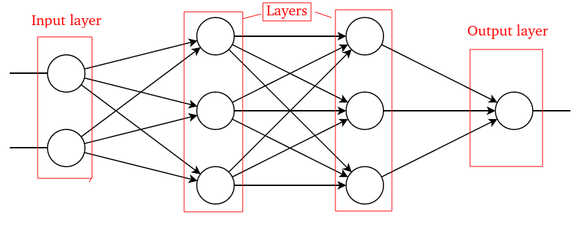
Layer

Open your code editor, create the file "neural_network.py" and write this.

class Layer:
    def __init__(self, neurons):
        self.neurons:int = neurons # the layer neurons
        self.shape:tuple = None # input shape
        self.W = None # the wight matrix, shape (inputs, neurons)
        self.B = None # the bias matrix,  shape (1, neurons)

    def forward(self, X): # output shape (input_examples, neurons)
        if self.shape is None:
            self.init_layer(X)
        return np.matmul(X, self.W) + self.B # matrix multiplication

    def init_layer(self, X):
        self.shape = (X.shape[-1], self.neurons) # X.shape (input_examples, input_data_size)
        # create initial parameters
        self.W = np.random.rand(*self.shape) * 2 - 1
        self.B = np.random.rand(1, self.neurons) * 2 - 1

    def __call__(self, X, training=False):
        Y = self.forward(X)
        if training: # if the model is training
            self.X = X
            self.Y = Y
        return Y

This is the implementation of a layer, a layer is a set of neurons receiving the same inputs

But, this is layers of linear functions, only it can do linear regressions.
For make a neural network, the layers need activation functions. we will implement it.

Activation function

First we implement the activation functions, this are the sigmoid activation and tanh activation
Sigmoid:

Tanh:

ReLU:

We implement it:

# a dict for select a activation function
activations = {
    'sigmoid': {
        'function': lambda X: 1 / (1 + np.e**(-X)),
        'derivative': lambda X: np.e**(-X) / ((1 + np.e**(-X))**2)
    },
    'tanh': {
        'function': lambda X: np.tanh(X),
        'derivative': lambda X: 1 - np.tanh(X) ** 2
    },
    'relu': {
        'function': lambda X: ((X / (X.max() + 1)) * (X > 0)),
        'derivative': lambda X: 1 * (X >= 0)
    }
}

Now, the Layer with activation function.

class Dense(Layer): # this inherits from the Layer class
    def __init__(self, neurons, activation='sigmoid'): # sigmoid activations for default
        super().__init__(neurons) # init the layer 
        self.activation:dict = activations[activation] # get specific activations functions

    def forward(self, X):
        Y = super().forward(X)
        return self.activation['function'](Y) # calculate with activations function

Neural Network Model

Finally, the neural network.

class Model:
    def __init__(self, layers:list=[]):
        self.layers:list = layers

    def add(self, layer: Layer):# add a Layer
        self.layers.append(layer)

    def forward(self, X, training=False): # forward in all layers
        Y = X
        for layer in self.layers:
            Y = layer(Y, training)
        return Y

    def __call__(self, X, training=False):
        return self.forward(X, training)

Testing our model.

In other file "test_model.py" copy this:

import unittest
import numpy as np
from neural_network import Dense, Layer, Model

def testing_model_outputs(model: Model, condition):
    examples: int = np.random.randint(512) + 1  # random number of examples between 1-512
    inputs: int = np.random.randint(256) + 1  # random number of inputs between 1-256
    X = np.random.rand(examples, inputs)
    Y = model(X)
    assertion = condition(X, Y)
    return assertion

def add_many_layers_to_model(model: Model, layer:Layer):
    layers = np.random.randint(10) + 1  # random number of layers between 1-10
    for _ in range(layers):
        neurons = np.random.randint(128) + 1
        model.add(layer(neurons))

class TestNeuralNetwork(unittest.TestCase):
    def test_model_without_layers(self):
        """
        The model has no intermediate layers, the input and output must be the same 
        because the data was processed
        """
        assert testing_model_outputs(
            Model([]),
            # input and output are the same, so their subtraction is 0
            condition=lambda X, Y: np.mean(Y - X) == 0
        )

    def test_model_number_of_examples_constant(self):
        """
        The input and the output are different but must have the same number of examples.
        If the input is from (m, i) the output must be from (m, n)
        """
        model = Model([])
        add_many_layers_to_model(model, Layer) # let's pass the Layer class as an argument
        assert testing_model_outputs(
            model,
            # X.shape[0] is the number of examples
            condition=lambda X, Y: Y.shape[0] == (X.shape[0])
        )

    def test_model_output_shape(self):
        """
        if you have an input with the form (m, i) and the last layer has "n" neurons, 
        the output must have the form (m, n)
        """
        model = Model([])
        add_many_layers_to_model(model, Layer) # let's pass the Layer class as an argument
        last_layer_neurons = 3
        model.add(Layer(last_layer_neurons))
        assert testing_model_outputs(
            model,
            # X.shape[0] is the number of examples of the input
            condition=lambda X, Y: Y.shape == (X.shape[0], last_layer_neurons)
        )
if __name__ == "__main__":
    unittest.main()

Don't panic!, this is just a test to see if the model works.
In this file 3 tests are carried out:

test_model_without_layers: the model has no layers, the input is not rendered, so the model returns the input as output.

test_model_number_of_examples_constant: the models have a random number of layers, but the number of examples must be the same, for example, if it receives 4 mathematical exercises it will deliver 4 mathematical exercises

test_model_output_shape: in the previous test we saw that the number of examples is constant, but each example must have the same number of outputs as the number of neurons in the last layer.

run:

python test_neural_network.py

output:

...
----------------------------------------------------------------------
Ran 3 tests in 0.009s
OK

This means it works. As an exercise you can add a method to the TestNeuralNetwork class and create a model with Dense layers, the model must return random values between 0-1
You can also initialize the Dense layers with a second argument "tanh" if the last layer has this parameter it will return values between -1 to 1

Training the model

We have the neural network implemented, now we need to train it.

Calculation of losses

We create a new file in the same folder "training_model.py" and we start typing this:

import time
import numpy as np

# we import our model
from neural_network import Model

def mse(Y, target):
    return np.mean((target - Y) ** 2, axis=1)

def d_mse(Y, target):
    return (2 * (Y - target)) / Y.shape[1]

"mse" mean square error, the error calculation model

• "m", is the output examples number.
• "t", targets
• "y", output prediction for the model

Calculation of gradients

Now type this in the same file:

def train_step(model: Model, X: np.ndarray, target: np.ndarray, lr: float):
Y = model(X, training=True) # model prediction
    acc = np.int64(target.argmax(axis=1) == Y.argmax(axis=1)).mean() # accuracy
    loss: np.ndarray = mse(Y, target) # prediction loss
    gradients = [] # gradients 
    for layer in reversed(model.layers): # Back-propagation
        derivative = layer.activation['derivative'] # activation derivative
        if layer == model.layers[-1]:
            fault: np.ndarray = d_mse(Y, target)
        # calculating the fault of the neuron
        fault = fault * derivative(layer.Y)
        # Gradient calculation
        gradient: np.ndarray = np.matmul(fault.T, layer.X).T
        b_gradient: np.ndarray = np.matmul(
            fault.T, np.ones((X.shape[0], 1))).T
        gradients.append((gradient, b_gradient)) # save to gradients
        # update fault for back layer
        fault: np.ndarray = np.matmul(fault, layer.W.T)

    for layer, gradient in zip(reversed(model.layers), gradients):
        gradient, b_gradient = gradient
        layer.W = layer.W - lr * gradient # Update weights
        layer.B = layer.B - lr * b_gradient # Update bias

    return loss.mean(), acc

Important functions and variables:

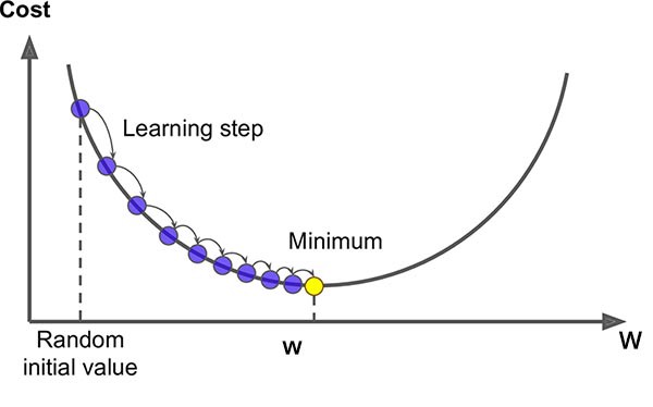
• gradient, is a vector that indicates where the new value of the weights "W" should move to
• b_gradient, gradients for the bias "B"
• update_parameters, this functions update the "W" and "B using the gradients"
• lr learning rate, is the step size that the weights "W" travel to approach the point of least loss

Gradient calculations are very complex. It is calculated in this way.

Training cycles

Type this code:

def fit(model: Model, X: np.ndarray, targets: np.ndarray,
        batch_size: int, epochs: int, learning_rate: float = 0.0001):
    # X and targets must have the same number of examples
    assert X.shape[0] == targets.shape[0]
    for epoch in range(epochs):

        last_examples = len(X) % batch_size
        # batching the inputs
        x = list(X[last_examples:].reshape(
            len(X) // batch_size, -1, X.shape[-1]))
        if X[:last_examples].size > 0:
            x.append(X[:last_examples])
        # batching the targets
        target = list(targets[last_examples:].reshape(
            len(X) // batch_size, -1, targets.shape[-1]))
        target.append(targets[:last_examples])
        # metrics variables
        error = None
        accuracy = None
        start = time.time()
        # epoch iteration
        print(f'Epoch: {epoch+1}:')
        for i, inp, tar in zip(range(len(x)), x, target):
            loss, acc = train_step(model, inp, tar, learning_rate)
            # metrics calculation
            if error is None and accuracy is None:
                error = loss
                accuracy = acc
            else:
                error = (error + loss) / 2
                accuracy = (accuracy + acc) / 2
            # printing metrics
            msg = f'batchs: {i+1}/{len(x)}, Error: {error} Acc: {acc}'
            print("", end='\r')
            print(msg, end='')
        print("", end='\r')
        print(msg + f' Time: {time.time() - start}')

Here we have the function "fit ", here we define the training cycles that our model will have, and some parameters to adjust.

• X is a matrix with the shape (m,i) contains the examples for the training of the model.
• targets are the expected outputs with the shape (m, n), "n" is the number of the outputs.
• batch_size is the size of the batch in which the examples are grouped, the data can be grouped in small batches to reduce the computational cost of training and help the model to generalize the information, if its value is 1 it will be trained the model sequentially.
• epochs is the number of times the model will cycle through all the examples
• learning_rate is already explaining

Testing our model with real data

Now we are going to use a jupyter notebook, if you aren't using vscode, you can code in a script.py
we create a file "test_model.ipynb" if you are using vscode or "test_model.py" if you use another code editor.
first we import what we need
We Install tensorflow to use a dataset and matplotlib to visualize the data.

pip install tensorflow matplotlib

# libraries
import numpy as np
from matplotlib import pyplot as plt
# Our code
from neural_network import Model, Dense
from training_model import fit, d_mse
# mnist dataset from tensorflow
from tensorflow.keras.datsets import mnist

Now we load the dataset

# Load dataset
(x_train, y_train), (x_test, y_test) = mnist.load_data()

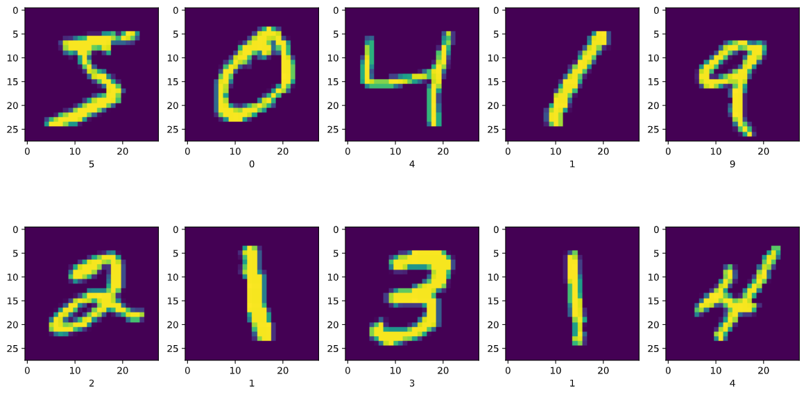
Viewing the dataset.

plt.figure(figsize=(15, 8))
for i, img, label in zip(range(10), x_train[:10], y_train[:10]):
    plt.subplot(2, 5, i + 1)
    plt.imshow(img)
    plt.xlabel(label)
plt.show()

If you managed to run the code until this point you should be able to view images of handwritten numbers.

Now we transform the data so that the model can process it.

x_train = x_train.reshape(len(x_train), -1) # shape (60000, 28*28)
x_train = x_train / 255 # normalizing data to values between 0-1
zeros = np.zeros(
    shape=(y_train.size, int(y_train.max() + 1)) # zeros matrix shape (m, i)
)
zeros[np.arange(len(y_train)), y_train] = 1 # one hot encodig
y_train = zeros # shape (60000, 10)

x_test = x_test.reshape(len(x_test), -1) # shape (10000, 28*28)
x_test = x_test / 255 # normalizing data to values between 0-1
zeros = np.zeros(
    shape=(y_test.size, int(y_test.max()) + 1) # zeros matrix shape (m, i)
)
zeros[np.arange(len(y_test)), y_test] = 1 # one hot encodig
y_test = zeros # shape (10000, 10)

We create the model:

model = Model([])
model.add(Dense(128, activation='relu'))
model.add(Dense(10, activation='sigmoid')) # output layer

The model has 2 layers, the hidden layer that has 128 neurons with the relu function and the output layer that has 10 neurons with the sigmoid function, the output layer will tell us what number it sees in each image.
Note that the number of neurons in the last layer is equal to the number of numerical characters that we have available in the dataset [0 1 2 3 4 5 6 7 8 9].
Now to train the model°

fit(model, x_train, y_train, batch_size=256, epochs=5, learning_rate=0.01)

Console output:

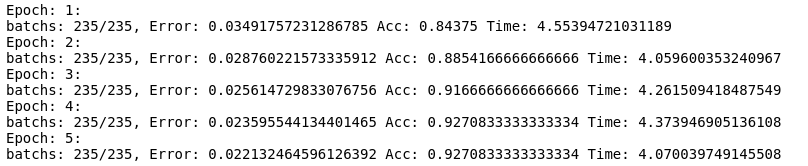
I explain:

• x_train is the input data for the model.
• y_train is the target, the expected output.
• batch_size the model loops through the dataset in batches of 256 samples.
• epoch 5 laps.
• learning_rate 0.01, The step size of the weights is small enough to avoid sudden changes in training.
  Apparently the model predicts with an acc = 0.9, that is, an accuracy of 90%. We will see if this is true using the test data.
  Type this in the file:

predictions = model(x_test)
ACC = np.int64(y_test.argmax(axis=1) == predictions.argmax(axis=1)).mean()
print (f'accuracy: {ACC}')

If the console output looks like this accuracy: 0.9063, the model was training correctly.
Try it with other values in the parameters of the fit function to see what results you can get. You can also try increasing more layers to the model with the number of neurons you want, the possible values for the "activation" parameter are the strings: "sigmoid ","tanh" and "relu".
Now we are going to visualize the test results with the test data
In the same file write:

def plot_image(i, predictions_array, true_label, img):
  predictions_array, true_label, img = predictions_array, true_label[i], img[i]
  plt.grid(False)
  plt.xticks([])
  plt.yticks([])
  plt.imshow(img, cmap=plt.cm.binary)
  predicted_label = np.argmax(predictions_array)
  true_label = np.argmax(true_label)
  if predicted_label == true_label:
    color = 'blue'
  else:
    color = 'red'
  plt.xlabel("{} {:2.0f}% ({})".format(predicted_label,
                                100*np.max(predictions_array),
                                true_label),
                                color=color)

def plot_value_array(i, predictions_array, true_label):
  predictions_array, true_label = predictions_array, true_label[i]
  plt.grid(False)
  plt.xticks(range(10))
  plt.yticks([])
  thisplot = plt.bar(range(10), predictions_array, color="#777777")
  plt.ylim([0, 1])
  predicted_label = np.argmax(predictions_array)
  true_label = np.argmax(true_label)
  thisplot[predicted_label].set_color('red')
  thisplot[true_label].set_color('blue')

And:

num_rows = 5
num_cols = 3
num_images = num_rows*num_cols
plt.figure(figsize=(2*2*num_cols, 2*num_rows))
for i in range(num_images):
  plt.subplot(num_rows, 2*num_cols, 2*i+1)
  plot_image(i, predictions[i], y_test, x_test.reshape(-1,28,28))
  plt.subplot(num_rows, 2*num_cols, 2*i+2)
  plot_value_array(i, predictions[i], y_test)
plt.tight_layout()
plt.show()

You should see a result like this.

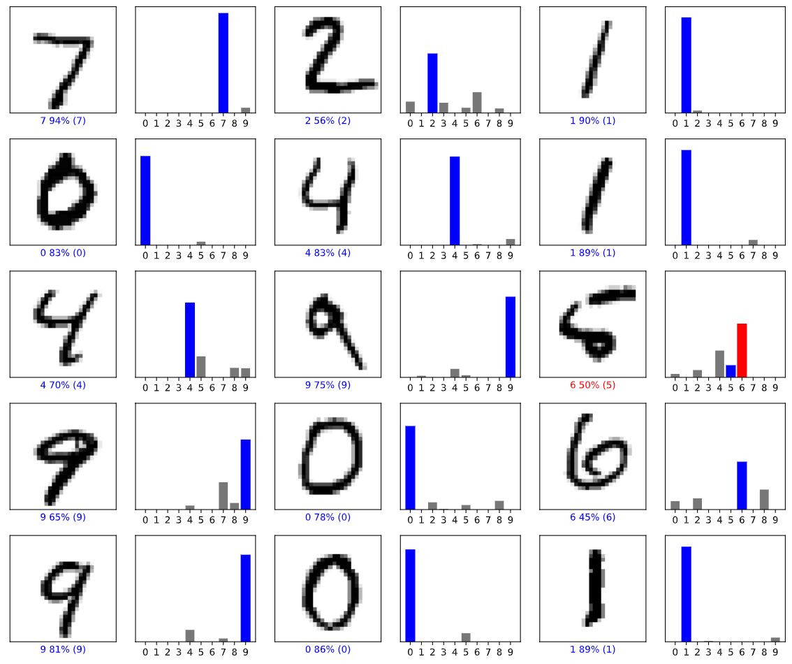
That's it, I hope you have learned something from this blog.
Bye.

Autor

• Willy samuel paz Colque

Source code

• github
• google colab